metaQuantome Command-line Tutorial
Caleb W. Easterly, Ray Sajulga, Subina Mehta, James Johnson, Praveen Kumar, Shane Hubler, Bart Mesuere, Joel Rudney, Timothy J. Griffin, Pratik D. Jagtap April 19, 2019
Introduction
This tutorial accompanies the article Easterly et al., Mol Cell Proteomics 2019, and is designed to show how to use the metaQuantome command line interface. An introduction to the metaQuantome Galaxy tool interface is available here.
Installing metaQuantome
The easiest way to install metaQuantome with all the dependencies is by using Bioconda (provided you are on Mac or Linux, which are the only systems supported by Bioconda).
First, install the conda package manager, by downloading either Anaconda or Miniconda (see https://docs.anaconda.com/anaconda/install/). Then, the following commands will set up the necessary channels for Bioconda and metaQuantome. If needed, additional information on Bioconda is available at https://bioconda.github.io/.
conda config --add channels defaults
conda config --add channels bioconda
conda config --add channels conda-forge
Then, run the following command to set up an environment named mqome, which will have metaQuantome (version 1.0.0) and all dependencies in it:
conda create -n mqome metaquantome=2.0.1
If the following prompt is seen at the command line, type y:
Proceeed ([y]/n)?
The create command only needs to be run once.
Finally, we can activate the environment using the following command, which will make the metaquantome command available.
source activate mqome
The rest of the tutorial will assume that you have the Conda environment activated, and are on a Mac or Linux system. Furthermore, you can follow along with the tutorial by cloning the Github repository at https://github.com/galaxyproteomics/metaquantome_mcp_analysis and changing your directory to <git_repo_root>/cli_tutorial. If you have any problems, please submit an issue at https://github.com/galaxyproteomics/metaquantome/issues.
The data
metaQuantome takes 2-3 input files depending on the mode of analysis. In the case of functional analysis, metaQuantome takes in a functional annotation file and a file with peptide intensities. For taxonomic analysis, the peptide intensity file and a file with lowest common ancestor (LCA) peptide annotations. For function-taxonomy interaction analysis, metaQuantome takes in all three files above.
In this tutorial, the data is from a previously published paper [1], and is downsampled in the interest of speed and simplicity - so, keep in mind that these results are by not necessarily representative. The purpose of this tutorial is to demonstrate the capabilities of metaQuantome, not to analyze the full dataset. We can see the beginning of each of the files below.
Function
| peptide | go |
|---|---|
| LPGQQHGTPSAK | GO:0009405,GO:0019867 |
| ELPGLAALTDK | GO:0006096,GO:0005737,GO:0004618,GO:0005524 |
| ELADASVSTIEIER | GO:0006412,GO:0015935,GO:0003735,GO:0019843,GO:0003729 |
| QISAGELR | GO:0006412,GO:0005840,GO:0022625,GO:0003735,GO:0003729 |
| VPAILADATK | GO:0055085 |
Note that there can be multiple GO terms (or no GO terms) annotated to a peptide, as long as they are separated by a comma.
Taxonomy
| peptide | lca |
|---|---|
| LPGQQHGTPSAK | Veillonella |
| ELPGLAALTDK | Bacteria |
| ELADASVSTIEIER | Bacteria |
| QISAGELR | Bacteria |
| VPAILADATK | Granulicatella adiacens |
Here, the peptides are annotated with their lowest common ancestor as a NCBI taxonomy names. Unlike names, NCBI taxIDs are unambiguous and not affected by differences in capitalization or spelling errors. So, taxIDs are highly recommended.
Peptide intensities
Here, the mass-spectrometer spectral intensities are provided for each peptide.
| peptide | X737WS | X737NS | X852WS | X852NS | X867WS | X867NS |
|---|---|---|---|---|---|---|
| LPGQQHGTPSAK | 160259.9 | 334347.7 | NA | NA | 564647.6 | 402888.9 |
| ELPGLAALTDK | 9640246.9 | NA | 6379355.0 | 1842767 | 5491673.7 | NA |
| ELADASVSTIEIER | 3957113.0 | NA | 238529.0 | NA | 1277833.8 | 165964.2 |
| QISAGELR | 17929965.5 | 774077.2 | 18109620.3 | 2481987 | 6576851.4 | NA |
| VPAILADATK | NA | 202338.2 | 447102.1 | 1892304 | 1049044.7 | 1696422.4 |
Note that missing data is here represented as NA. In general, metaQuantome treats 0, NA, and NaN as missing data.
Also, metaQuantome assumes that input data is untransformed and normalized - that is, the data should be on the original measurement scale (not log transformed or any other transformation), and it should be normalized by an appropriate method.
Databases
metaQuantome has a separate module for downloading the necessary databases. Let’s first get the helptext for the module and make sure everything is installed correctly:
metaquantome db -h
usage: metaquantome db [-h] [--dir DIR] [--update]
                       {ncbi,go,ec} [{ncbi,go,ec} ...]

positional arguments:
  {ncbi,go,ec}       database to download. note that COG mode does not require
                     a download due to its simplicity.

optional arguments:
  -h, --help         show this help message and exit
  --dir DIR, -d DIR  data directory for files.
  --update, -u       overwrite existing databases if present.
If you get any errors that suggest that there has been trouble installing the package, please post on https://github.com/galaxyproteomics/metaquantome/issues.
Now, to actually download the databases, choose a folder - here, data - and run the following command:
mkdir -p ./data
metaquantome db ncbi go --dir ./data
As detailed in the manuscript, the are several questions that metaQuantome can be used to explore. Let’s go through a few of these.
Most Abundant Taxa
metaQuantome can be used to identify the most abundant taxa in an experiment, and stratify this by condition. The workflow here is
expandthe set of annotations to include indirect annotationsfilterthe expanded results to well-supported taxavizthe filtered taxa, ranked by abundance.
Expand
metaQuantome requires information about each of the samples, and which experimental conditions they belong to. The names of the samples also should be the column names in the intensity file. For example, if you have two experimental conditions “A” and “B”, each with two samples that you’re calling “A1”, “A2”, and “B1”, “B2”, respectively, the columns of your intensity file should be peptide (or another peptide column name), A1,A2,B1, and B2. Then, the --samps argument gives metaQuantome the information about which samples below to which groups. There are two ways to provide this information to metaQuantome:
- a JSON string
- a tabular file
An example of the required tabular file is in input_files/samples.tab:
cat input_files/samples.tab
group   colnames
NS  X737NS,X852NS,X867NS
WS  X737WS,X852WS,X867WS
The file must have the ‘group colnames` header, and cannot end with a newline. Moreover, it must be separated with ‘hard’ tabs rather than ‘soft tabs’, as must all files used by metaQuantome - the easiest way to ensure this is to create the file in Excel or other spreadsheet software, and then export to a tab-separated file. On the other hand, the JSON option is simpler for a smaller number of samples. The JSON equivalent in this case is
'{"NS": ["X733NS","X852NS","X866NS"], "WS": ["X733WS", "X852WS", "X866WS"]}'
Note that the items in the JSON string must be surrounded by double quotes (e.g., "thing").
Now, let’s run the expand module on the files in input_files.
metaquantome expand \
    --mode t \
    --int_file input_files/int.tab \
    --pep_colname_int peptide \
    --tax_file input_files/tax.tab \
    --pep_colname_tax peptide \
    --tax_colname lca \
    --samps input_files/samples.tab \
    --outfile mqome_outputs/tax_expanded.tab \
    --data_dir data
Note that many of the arguments give column names in the input files, so that metaQuantome can keep track of what’s what. Specifically, it needs to know the name of the peptide column in each file (--pep_colname_int, --pep_colname_tax), and the name of the taxonomy least common ancestor column in the taxonomy file (tax_colname).
Let’s look at the output in mqome_outputs:
| id | taxon\_name | rank | NS\_mean | WS\_mean | X737NS | X737WS | X852NS | X852WS | X867NS | X867WS | X737NS\_n\_peptide | X737WS\_n\_peptide | X852NS\_n\_peptide | X852WS\_n\_peptide | X867NS\_n\_peptide | X867WS\_n\_peptide | X737NS\_n\_samp\_children | X737WS\_n\_samp\_children | X852NS\_n\_samp\_children | X852WS\_n\_samp\_children | X867NS\_n\_samp\_children | X867WS\_n\_samp\_children |
|---|---|---|---|---|---|---|---|---|---|---|---|---|---|---|---|---|---|---|---|---|---|---|
| 481 | Neisseriaceae | family | 21.18733 | 16.54774 | 22.09506 | 17.25113 | 18.17465 | 15.11985 | NA | NA | 1 | 1 | 1 | 1 | NA | NA | 1 | 1 | 1 | 1 | NA | NA |
| 538 | Eikenella | genus | 21.18733 | 16.54774 | 22.09506 | 17.25113 | 18.17465 | 15.11985 | NA | NA | 1 | 1 | 1 | 1 | NA | NA | 1 | 1 | 1 | 1 | NA | NA |
| 539 | Eikenella corrodens | species | 21.18733 | 16.54774 | 22.09506 | 17.25113 | 18.17465 | 15.11985 | NA | NA | 1 | 1 | 1 | 1 | NA | NA | NA | NA | NA | NA | NA | NA |
| 712 | Pasteurellaceae | family | 26.45509 | 24.24076 | 24.96501 | 22.21824 | NA | 17.34137 | 27.1723 | 25.69783 | 12 | 12 | NA | 1 | 12 | 12 | 1 | 1 | NA | NA | 1 | 1 |
| 724 | Haemophilus | genus | 26.04355 | 24.30867 | 23.49238 | 21.57275 | NA | NA | 26.9149 | 25.19611 | 5 | 5 | NA | NA | 5 | 5 | 1 | 1 | NA | NA | 1 | 1 |
(The software used to write this tutorial puts in the backslashes (\) in the column names - those aren’t actually there in the file)
Quantitative outputs are included (columns like “NS_mean”, which shows the log base 2 of the average intensity for that term), as well as information about the ‘quality’ of the annotations, like “X733NS_n_peptide”, which shows the number of peptides that give evidence for each term. For example, 4 peptides were observed in sample X733NS that were annotated with the Firmicutes phylum or any of its children. These extra columns are included because they are used in metaquantome filter, and for the sake of transparency.
Filter
Now, let’s filter the expanded outputs to terms about which we have a certain level of confidence.
metaquantome filter \
    --expand_file mqome_outputs/tax_expanded.tab \
    --mode t \
    --samps input_files/samples.tab \
    --min_peptides 1 \
    --min_pep_nsamp 1 \
    --min_children_non_leaf 2 \
    --min_child_nsamp 1 \
    --qthreshold 2 \
    --outfile mqome_outputs/tax_filt.tab
Here, we’re requiring that each term satisfy the following conditions:
- Evidenced by at least 1 peptide in at least 1 sample of each group
- Has 0 sample children (leaf) or at least 2 sample children in at least 1 sample of each group (see paper for definition of sample children)
- Was quantified in at least 2 samples of each group
Let’s look at the output:
| id | taxon\_name | rank | NS\_mean | WS\_mean | X737NS | X737WS | X852NS | X852WS | X867NS | X867WS | X737NS\_n\_peptide | X737WS\_n\_peptide | X852NS\_n\_peptide | X852WS\_n\_peptide | X867NS\_n\_peptide | X867WS\_n\_peptide | X737NS\_n\_samp\_children | X737WS\_n\_samp\_children | X852NS\_n\_samp\_children | X852WS\_n\_samp\_children | X867NS\_n\_samp\_children | X867WS\_n\_samp\_children |
|---|---|---|---|---|---|---|---|---|---|---|---|---|---|---|---|---|---|---|---|---|---|---|
| 712 | Pasteurellaceae | family | 26.45509 | 24.24076 | 24.96501 | 22.21824 | 0.00000 | 17.34137 | 27.17230 | 25.69783 | 12 | 12 | 0 | 1 | 12 | 12 | 1 | 1 | 0 | 0 | 1 | 1 |
| 724 | Haemophilus | genus | 26.04355 | 24.30867 | 23.49238 | 21.57275 | 0.00000 | 0.00000 | 26.91490 | 25.19611 | 5 | 5 | 0 | 0 | 5 | 5 | 1 | 1 | 0 | 0 | 1 | 1 |
| 729 | Haemophilus parainfluenzae | species | 23.51605 | 21.83745 | 22.11308 | 20.13283 | 0.00000 | 0.00000 | 24.21369 | 22.59720 | 4 | 4 | 0 | 0 | 4 | 4 | 0 | 0 | 0 | 0 | 0 | 0 |
| 1224 | Proteobacteria | phylum | 26.50641 | 26.40567 | 25.64756 | 25.68405 | 25.57253 | 26.02080 | 27.45138 | 27.10854 | 18 | 18 | 3 | 4 | 17 | 17 | 2 | 2 | 2 | 2 | 2 | 2 |
| 1239 | Firmicutes | phylum | 28.51239 | 30.09143 | 28.16821 | 29.85861 | 28.68930 | 29.90299 | 28.62579 | 30.43794 | 247 | 362 | 325 | 366 | 317 | 354 | 3 | 2 | 3 | 3 | 3 | 2 |
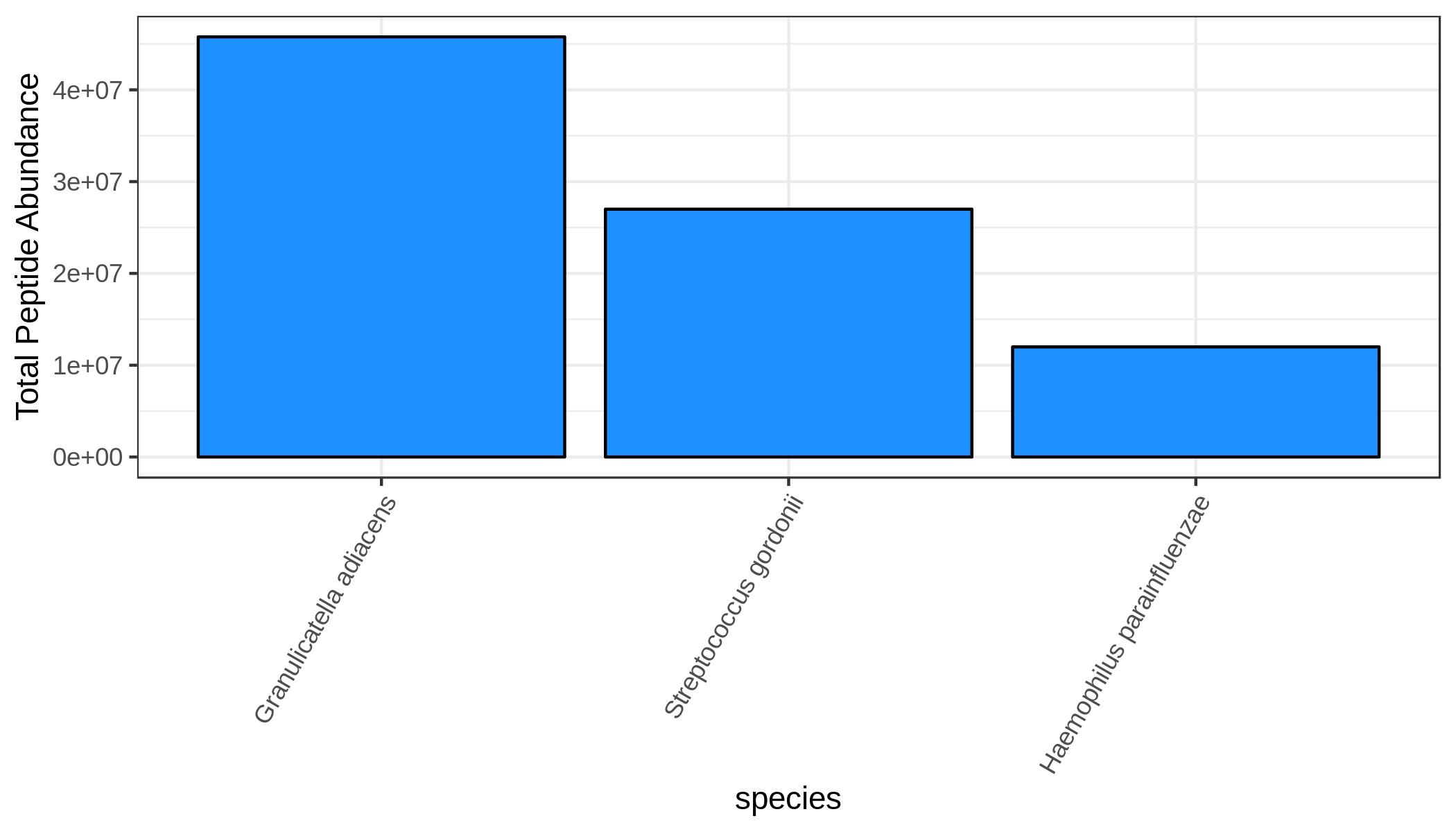
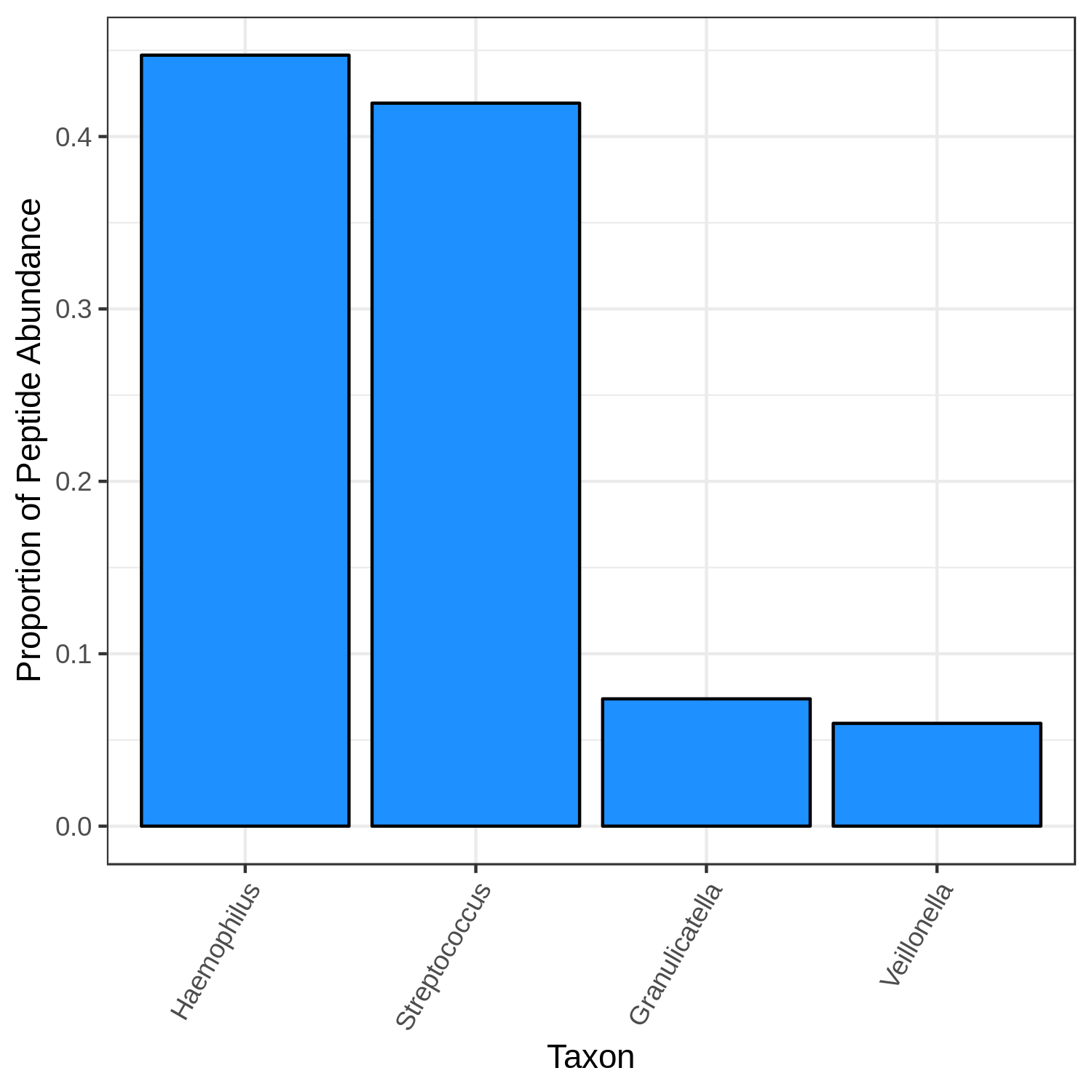
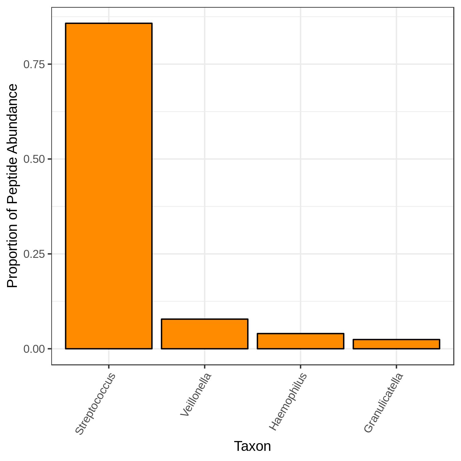
Viz
Finally, using the filtered output, we can visualize the most abundant taxa with the viz module. To do this, we provide viz with the name of the mean column (or any column) and a few other arguments. The most important argument for visualizing taxonomy is --target_rank, which indicates the rank we want to see. Let’s go with species for now (since it’s a reduced dataset, there aren’t that many genera or families or so on). In addition, we can choose the number of terms we want to display (--nterms).
metaquantome viz \
    --plottype bar \
    --infile mqome_outputs/tax_filt.tab \
    --mode t \
    --samps input_files/samples.tab \
    --meancol NS_mean \
    --target_rank species \
    --nterms 3 \
    --img mqome_outputs/imgs/tax_ns.png \
    --width 7 \
    --height 4 \
    --barcol 1
metaquantome viz \
    --plottype bar \
    --infile mqome_outputs/tax_filt.tab \
    --mode t \
    --samps input_files/samples.tab \
    --meancol WS_mean \
    --target_rank species \
    --nterms 3 \
    --img mqome_outputs/imgs/tax_ws.png \
    --width 7 \
    --height 4 \
    --barcol 2
NS
WS

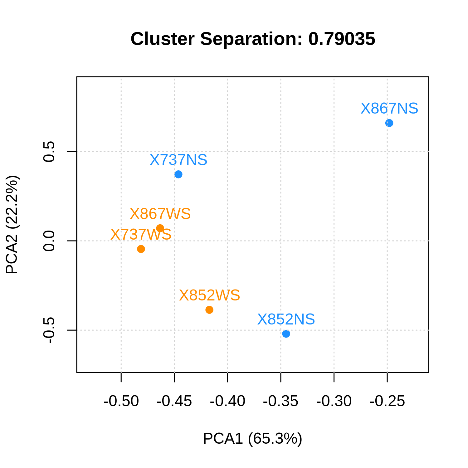
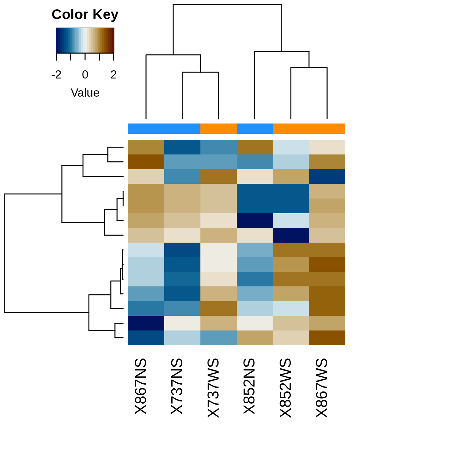
Cluster Analysis of Taxonomy
metaQuantome offers two methods for cluster analysis: principal components analysis and hierarchically clustered heatmaps. In both cases, we can use the mqome_outputs/tax_filt.tab file already produced above in the expand and filter steps.
Principal components analysis
metaquantome viz \
    --plottype pca \
    --infile mqome_outputs/tax_filt.tab \
    --mode t \
    --samps input_files/samples.tab \
    --img mqome_outputs/imgs/tax_pca.png \
    --calculate_sep
The --calculate_sep argument tells metaQuantome to calculate the ratio of the between-cluster variance to the within-cluster variance, where higher indicates a better separation of clusters (see the main paper for details). The separation is included in the plot title.
Heatmap
metaquantome viz \
    --plottype heatmap \
    --infile mqome_outputs/tax_filt.tab \
    --mode t \
    --samps input_files/samples.tab \
    --img mqome_outputs/imgs/tax_heatmap.png
Differentially Abundant Functions
Now, let’s go through a differential abundance analysis with metaQuantome. We’ll do analysis on GO terms, and look for terms that are significantly different between the no sucrose (NS) and with sucrose (WS) samples. The workflow is similar, but we add another step (stat), so we do expand -> filter -> stat -> viz.
Expand
metaquantome expand \
    --mode f \
    --data_dir data \
    --int_file input_files/int.tab \
    --pep_colname_int peptide \
    --func_file input_files/func.tab \
    --pep_colname_func peptide \
    --func_colname go \
    --ontology go \
    --samps input_files/samples.tab \
    --outfile mqome_outputs/func_expanded.tab
Filter
Here, we filter to GO terms with good evidence, and those that are appropriate for statistical analysis. Specifically, we need at least 3 samples per group for a robust t-test.
metaquantome filter \
    --expand_file mqome_outputs/func_expanded.tab \
    --mode f \
    --ontology go \
    --samps input_files/samples.tab \
    --min_peptides 2 \
    --min_pep_nsamp 2 \
    --min_children_non_leaf 2 \
    --min_child_nsamp 2 \
    --qthreshold 3 \
    --outfile mqome_outputs/func_filt.tab
Stat
In stat, we use the tabular result from filter to append fold changes and the p-values obtained from t-tests. For additional options, use metaquantome stat -h
metaquantome stat \
    --file mqome_outputs/func_filt.tab \
    --mode f \
    --ontology go \
    --samps input_files/samples.tab \
    --parametric True \
    --paired \
    --outfile mqome_outputs/func_stat.tab
Viz
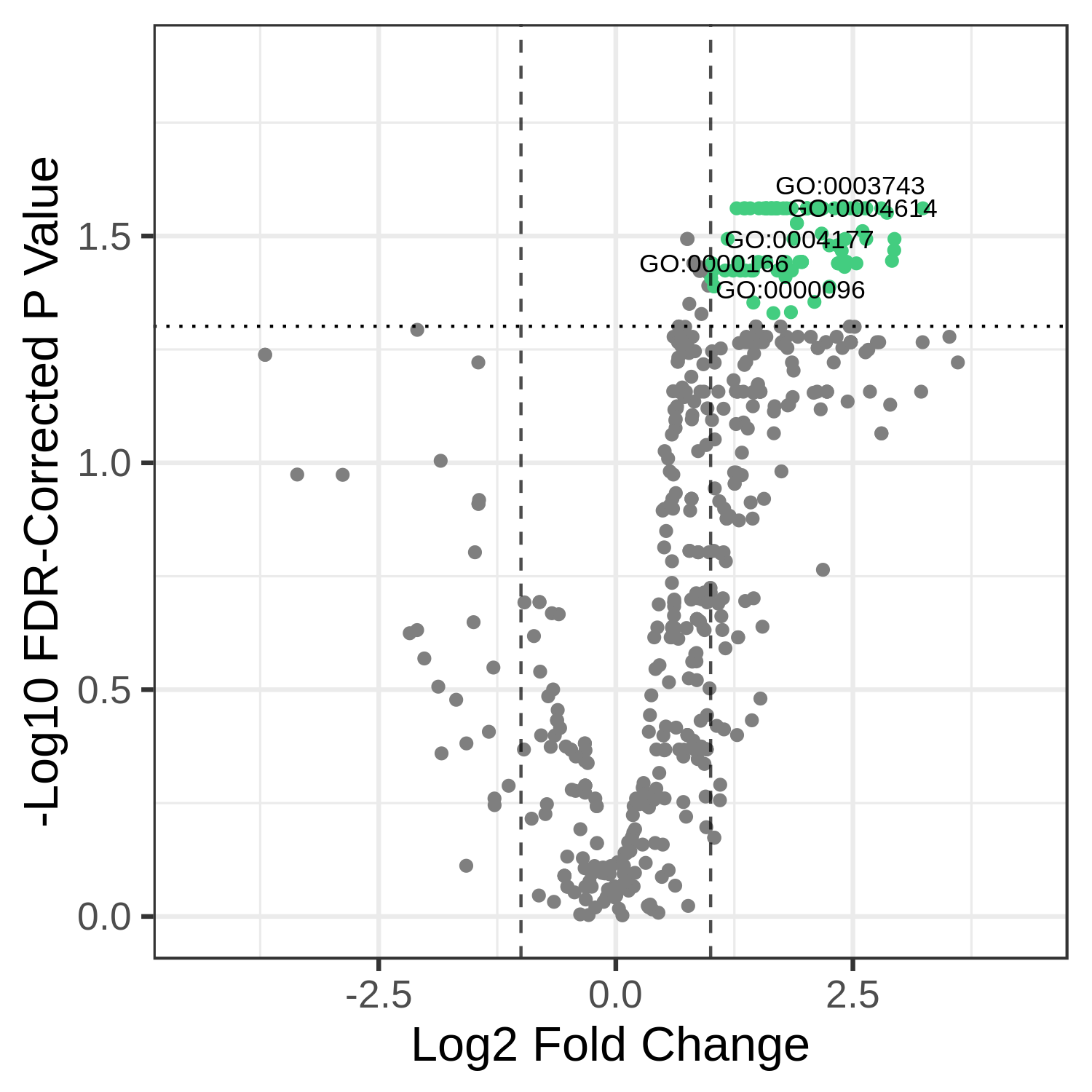
The visualization provided by metaQuantome for differential abundance is a volcano plot, where the -log10 p value is plotted against the log2 fold change.
Here, we provide the name of the fold change column in the result from stat, and whether or not to reverse the fold change. Note that the fold change is automatically calculated by alphabetizing the two group names, so we may want to reverse the order (here, we want to know WS over NS rather than NS over WS).
metaquantome viz \
    --plottype volcano \
    --infile mqome_outputs/func_stat.tab \
    --mode f \
    --samps input_files/samples.tab \
    --meancol NS_mean \
    --fc_name log2fc_NS_over_WS \
    --flip_fc \
    --img mqome_outputs/imgs/func_dea.png
We may also want to see the names specific terms that are differentially abundant. To do this, we provide the name of the column that has the text we want to plot - usually, the id column (for function) or taxon_name (for taxonomy) to --textannot. The plotting program automatically hides some of the terms to avoid overplotting - see mqome_outputs/func_stat.tab for the full list of results.
metaquantome viz \
    --plottype volcano \
    --infile mqome_outputs/func_stat.tab \
    --mode f \
    --samps input_files/samples.tab \
    --meancol NS_mean \
    --fc_name log2fc_NS_over_WS \
    --flip_fc \
    --img mqome_outputs/imgs/func_dea_text.png \
    --textannot id
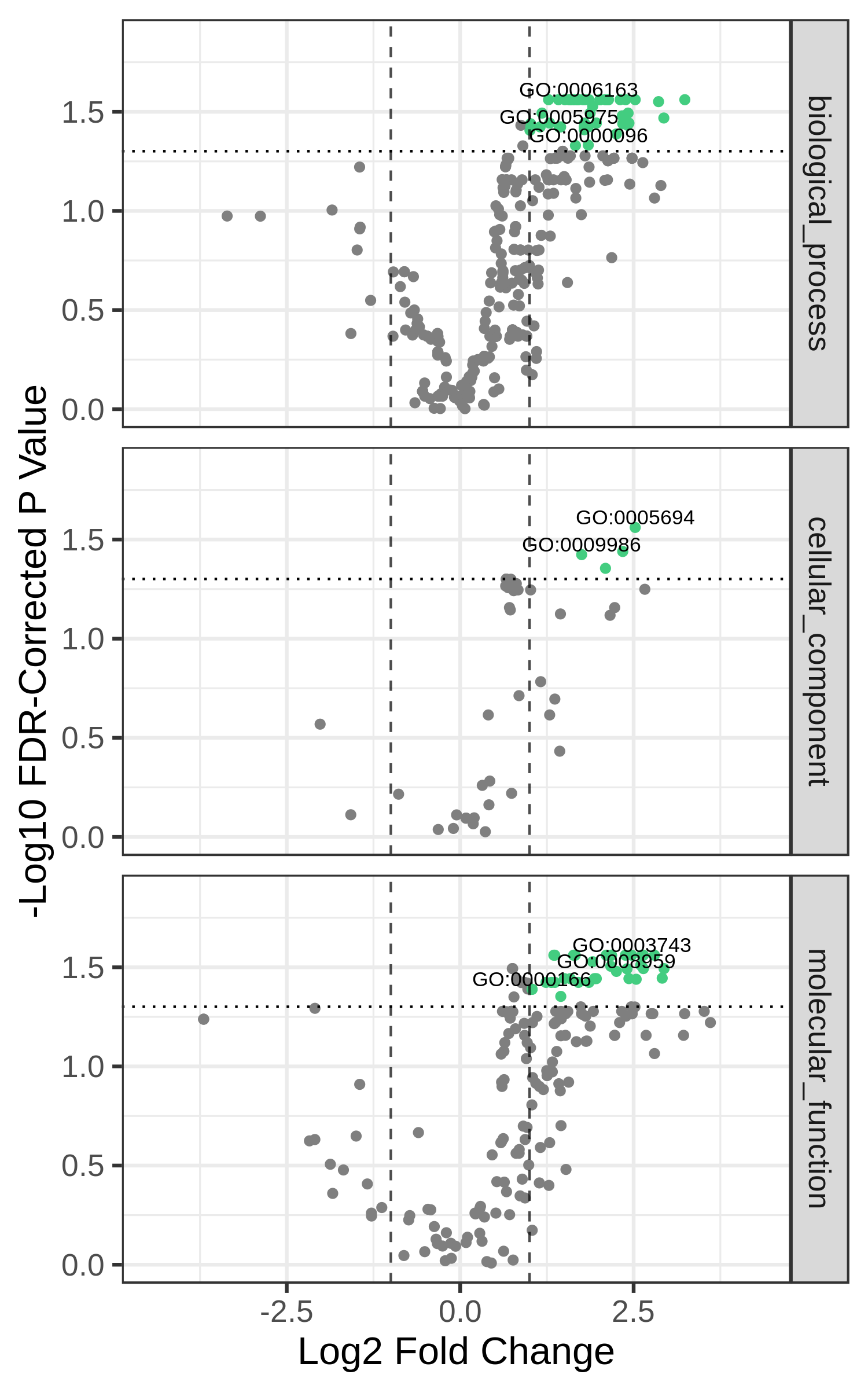
Finally, we may also want to divide the GO terms by ontology - biological process, molecular function, and cellular component. We can do that by providing the flag --gosplit. You may also have to tweak the --width and --height (in inches) to get everything looking right.
metaquantome viz \
    --plottype volcano \
    --infile mqome_outputs/func_stat.tab \
    --mode f \
    --samps input_files/samples.tab \
    --meancol NS_mean \
    --fc_name log2fc_NS_over_WS \
    --flip_fc \
    --img mqome_outputs/imgs/func_dea_text_split.png \
    --textannot id \
    --gosplit \
    --width 5 \
    --height 8
Function-Taxonomy Interaction
In this analysis, we examine the contribution of each taxon to carbohydrate metabolism, which is denoted by the GO term GO:0005975, “carbohydrate metabolic process”. Once again, the workflow is expand -> filter, but now we go straight to viz (testing is not recommended in function-taxonomy interaction mode).
Expand
First, we run the expand module. The mode is now ft, and we have to provide information about each of the intensity, taxonomy, and function files.
metaquantome expand \
    --mode ft \
    --data_dir data \
    --int_file input_files/int.tab \
    --pep_colname_int peptide \
    --tax_file input_files/tax.tab \
    --pep_colname_tax peptide \
    --tax_colname lca \
    --func_file input_files/func.tab \
    --pep_colname_func peptide \
    --func_colname go \
    --ontology go \
    --samps input_files/samples.tab \
    --outfile mqome_outputs/ft_expanded.tab
Filter
Now, we run the filter module, which does not change much by mode.
metaquantome filter \
    --expand_file mqome_outputs/ft_expanded.tab \
    --mode ft \
    --samps input_files/samples.tab \
    --min_peptides 1 \
    --min_pep_nsamp 1 \
    --min_children_non_leaf 2 \
    --min_child_nsamp 1 \
    --qthreshold 2 \
    --outfile mqome_outputs/ft_filt.tab
Viz
Finally, we visualize the results. Many vizualizations can be made from the same filter result file, including looking at taxonomic distribution of a functional term (--whichway t_dist) and looking at the functional distribution for a taxon (--whichway f_dist). In addition, for t_dist we need to provide the --target_rank; that is, the rank for which we’re interested in the distribution. Here, the target rank is genus.
metaquantome viz \
    --mode ft \
    --samps samples.tab \
    --infile mqome_outputs/ft_filt.tab \
    --img mqome_outputs/imgs/ft_carbo_ns.png \
    --plottype ft_dist \
    --meancol NS_mean \
    --whichway t_dist \
    --id GO:0005975 \
    --target_rank genus \
    --nterms all \
    --barcol 1
metaquantome viz \
    --mode ft \
    --samps samples.tab \
    --infile mqome_outputs/ft_filt.tab \
    --img mqome_outputs/imgs/ft_carbo_ws.png \
    --plottype ft_dist \
    --meancol WS_mean \
    --whichway t_dist \
    --id GO:0005975 \
    --target_rank genus \
    --nterms all \
    --barcol 2
NS
WS
The End
Thank you for going through the tutorial! As we mentioned above, use the help flag for full documentation of each command (e.g. metaquantome expand -h), and, if you have any problems or questions, submit an issue at https://github.com/galaxyproteomics/metaquantome/issues